For simplicity, we wrote PDEs in vector form, but they can also be expressed in component, e.g. \[
-\nabla \cdot (k\nabla u) = -\partial_x(k \partial_x u) - \partial_y(k \partial_y u) - \partial_z(k \partial_z u).
\]
Domain \(\Omega\) with boundary \(\Gamma\), the domain \(\Omega\) is where the PDE holds. (Mathematically, a domain is an open, non-empty, connected subset of \(\mathbb{R}^n\) (e.g., a 2D region or 3D volume), and the boundary is its edge)
\(\Gamma = \partial \Omega\) is where we specify boundary conditions, \(n\) is the outward normal vector on \(\Gamma\).
Boundary conditions:
Dirichlet: \(u = u_D\) on \(\Gamma_D\) (specify value of \(u\))
Neumann: \(-k\nabla u \cdot n = g_N\) on \(\Gamma_N\) (specify flux across boundary)
Robin: \(\alpha u + \beta (-k\nabla u \cdot n) = g_R\) on \(\Gamma_R\) (combination of value and flux)
A BVP: \[
\begin{cases}
-\nabla \cdot (k\nabla u) = f & \text{in } \Omega, \\
u = u_D & \text{on } \Gamma_D, \\
-k\nabla u \cdot n = g_N & \text{on } \Gamma_N.
\end{cases}
\]
1.3 Exact solution
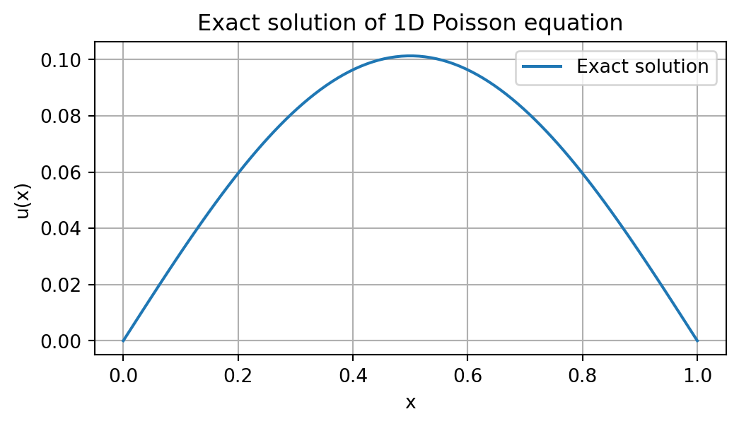
For some simpler BVPs, we can find an exact solution analytically. \[
-\partial_x(k \partial_x u) = f(x) \quad \text{on } (0,1),
\qquad u(0)=u(1)=0.
\] with constant \(k \in \mathbb{R}, k \neq 0\) and \(f = \sin(\pi x)\) has exact solution:
\[
u(x) = \tfrac{\sin(\pi x)}{k\pi^2}.
\]
Since \(\partial_x(k \partial_x u) = \partial_x\left(k \frac{\pi \cos(\pi x)}{k\pi^2}\right) = -\sin(\pi x)\), and the BCs are satisfied.
import numpy as npimport matplotlib.pyplot as pltx = np.linspace(0, 1, 100)k =1.0u = np.sin(np.pi * x) / (k * np.pi**2)plt.plot(x, u, label='Exact solution')plt.xlabel('x')plt.ylabel('u(x)')plt.title('Exact solution of 1D Poisson equation')# change sizeplt.gcf().set_size_inches(6, 3)plt.grid(); plt.legend(); plt.show()
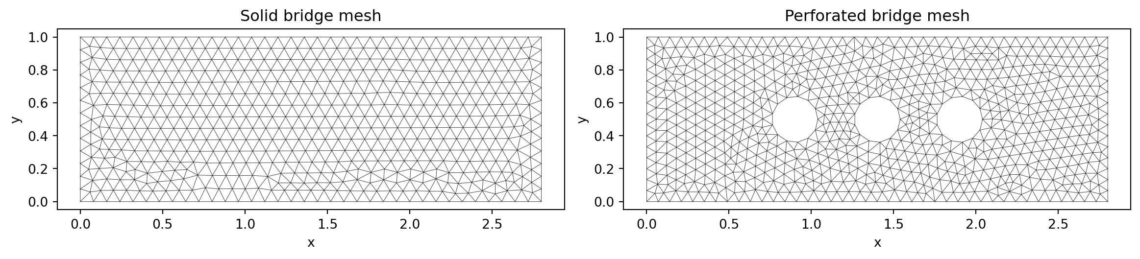
1.4 More complex domains
For structured domains, the finite difference method (see exercise) can sometimes help.
However, for more complex domains (e.g., with holes, curved boundaries), we need a more flexible method.
Finite element method (FEM): Can handle complex domains, unstructured meshes, and variable coefficients.
Mesh example
Note
The starting point for FEM is a weak (variational) formulation of the PDE.
2 Weak forms
For a given PDE (strong form), e.g., the Poisson equation with mixed BCs: \[
-\nabla \cdot (k\nabla u) = f \quad \text{in } \Omega, \qquad u = u_D \text{ on } \Gamma_D, \qquad -k\nabla u\cdot n = g_N \text{ on } \Gamma_N
\]
multiply by a test function \(v\) and integrate over \(\Omega\) to get the weak form: \[
\int_\Omega -\nabla \cdot (k\nabla u) v\,dx = \int_\Omega f v\,dx.
\]
Apply integration by parts to move derivatives from \(u\) to \(v\): \[
\int_\Omega k\nabla u \cdot \nabla v\,dx - \int_{\Gamma_N} \left(k\nabla u \cdot n\right) v\,ds
= \int_\Omega f v\,dx
\]
Insertion of Neumann BC: \[
\int_\Omega k\nabla u \cdot \nabla v\,dx
= \int_\Omega f v\,dx + \int_{\Gamma_N} g_N v\,ds.
\]
2.1 Variational problem
Define trial space \(V\) and test space \(V_0\)
Sobolev space \(H^1(\Omega)\) include functions with square-integrable derivatives, i.e., \(H^1(\Omega) = \{ w\in L^2(\Omega)\,|\,\nabla w \in (L^2(\Omega))^d \}\) meaning \(w\) and its gradient are square-integrable, i.e., \(\int_\Omega |w|^2\,dx < \infty\) and \(\int_\Omega |\nabla w|^2\,dx < \infty\). \[
V = \{ w\in H^1(\Omega)\,|\,w=u_D\text{ on }\Gamma_D\}, \qquad
V_0 = \{ w\in H^1(\Omega)\,|\,w=0\text{ on }\Gamma_D\}.
\]
Resulting problem: Find \(u\in V\) such that
\[
a(u,v)=L(v)\quad \forall v\in V_0,
\]
with a form \(a : V \times V_0 \to \mathbb{R}\) and a linear form \(L: V_0 \to \mathbb{R}\) defined as
Energy minimization (calculus of variations): \(\min_{u\in H_0^1(\Omega)} E(u)\) leads to \(E'(u;v) = 0\) for all “direction” \(v\in V_0\) as the first-order optimality condition, which is exactly the weak form.
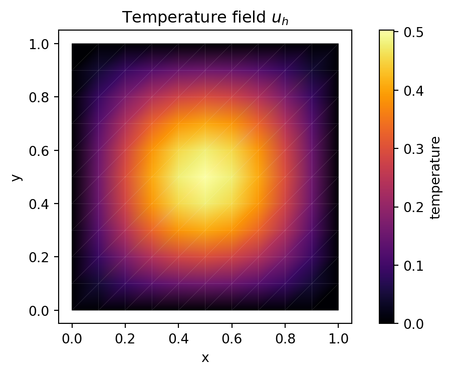
Therefore, \(u_h = \sum_{j=1}^N U_j\phi_j\) with basis functions \(\{\phi_j\}\) of \(V_h\) and unknown coefficients \(U_j\).
Inseration into the variational form and testing with basis \(\phi_i\) leads to: \[
\sum_{j=1}^N U_j a(\phi_j, \phi_i) = L(\phi_i) \quad \forall i=1,\ldots,N,
\]
2.4 Coefficient equation
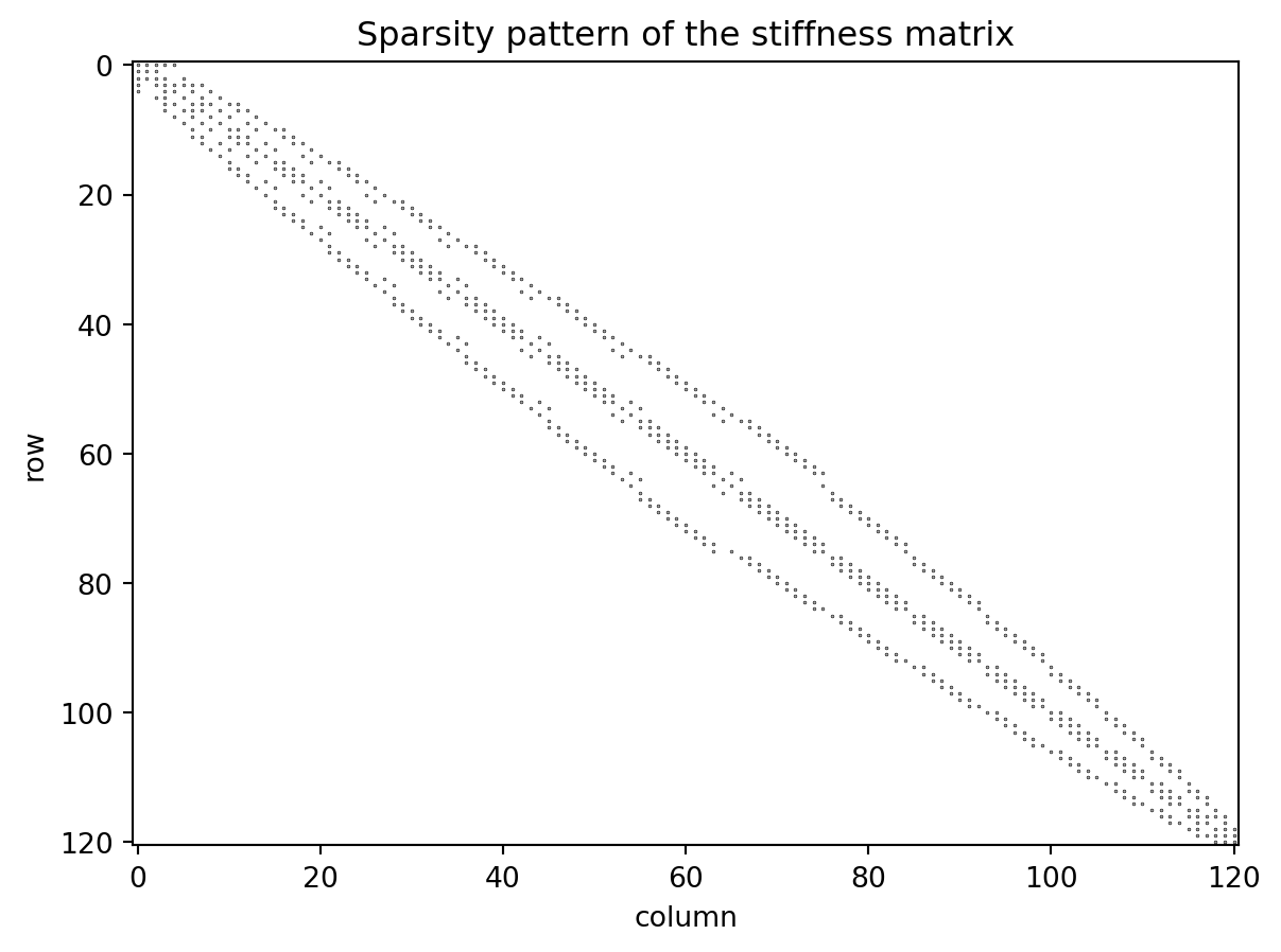
Linear system of equations: \[
\boldsymbol{A}\boldsymbol{U} = \boldsymbol{b} \quad \Leftrightarrow \quad \sum_{j=1}^N A_{ij}U_j = b_i \quad \forall i=1,\ldots,N,
\] with \(A_{ij} = a(\phi_j, \phi_i) = \int_\Omega \nabla \phi_j \cdot \nabla \phi_i\,dx\) and \(b_i = L(\phi_i) = \int_\Omega f\phi_i\,dx\).
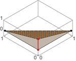
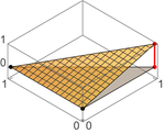
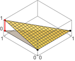
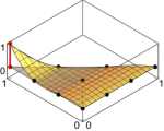
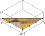
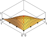
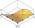
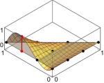
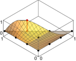
P1 (linear) elements have 3 nodes per triangle (vertices)
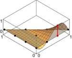
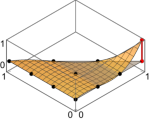
P3 Lagrange elements (cubic polynomials) have more nodes and higher-order basis functions, leading to better accuracy but also larger linear systems.
P3 Lagrange 1
P3 Lagrange 2
P3 Lagrange 3
P3 Lagrange 4
P3 Lagrange 5
P3 Lagrange 6
P3 Lagrange 7
P3 Lagrange 8
P3 Lagrange 9
3 FEniCS framework
FEniCS automates the whole process: from mesh generation, function space construction, variational form definition, assembly, to solving linear systems.
UFL: The Unified Form Language is a domain-specific language to formulate problems. It serves as the input for the form compiler.
FFCX: The FEniCS Form Compiler automatically generates DOLFIN code from a given variational form. The goal of a form compileris to use a well-tested compiler, performing automated code generation tasks, in order to improve the correctness of the resulting code.
BASIX/FIAT: The FInite element Automatic Tabulator enables the automatic computation of basis functions for nearly arbitrary finite elements.
3.1 Elements and forms
FEniCS supports a wide range of finite elements (Lagrange, Raviart–Thomas, Nédélec, etc.), see BASIX
UFL allows to express variational forms (linear, nonlinear, time-dependent), for example:
u = ufl.TrialFunction(V)v = ufl.TestFunction(V)a = k * ufl.dot(ufl.grad(u), ufl.grad(v)) * ufl.dxL = f * v * ufl.dx + g_N * v * ulf.ds
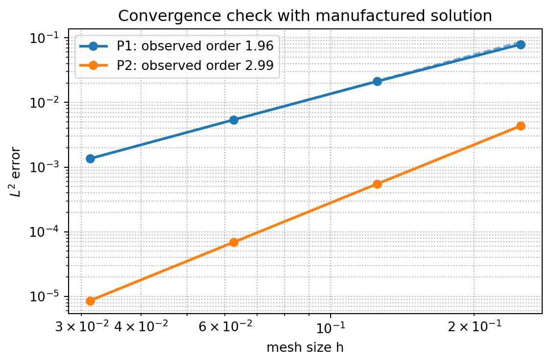
To verify an FEM implementation, we often use a manufactured solution: choose a smooth exact solution \(u_{\mathrm{ex}}\), insert it into the PDE, and derive the matching right-hand side \(f\).
For the Poisson problem on \(\Omega = (0,1)^2\), take
with homogeneous Dirichlet boundary conditions. Since \(u_{\mathrm{ex}}=0\) on \(\partial\Omega\), it fits the same setup as before. For smooth solutions, we expect the \(L^2\) error to behave like \(O(h^{p+1})\) for Lagrange elements of degree \(p\).
def solve_manufactured_problem(n, degree): msh = mesh.create_unit_square(MPI.COMM_WORLD, n, n) V = fem.functionspace(msh, ("Lagrange", degree)) u = ufl.TrialFunction(V) v = ufl.TestFunction(V) x = ufl.SpatialCoordinate(msh) u_exact = ufl.sin(ufl.pi * x[0]) * ufl.sin(ufl.pi * x[1]) f =2.0* ufl.pi**2* u_exact a = ufl.dot(ufl.grad(u), ufl.grad(v)) * ufl.dx L = f * v * ufl.dx fdim = msh.topology.dim -1 boundary_facets = mesh.locate_entities_boundary( msh, fdim,lambda x: np.isclose(x[0], 0.0)| np.isclose(x[0], 1.0)| np.isclose(x[1], 0.0)| np.isclose(x[1], 1.0), ) dofs = fem.locate_dofs_topological(V, fdim, boundary_facets) bc = fem.dirichletbc(PETSc.ScalarType(0.0), dofs, V) linear_problem_kwargs = {"petsc_options": {"ksp_type": "preonly", "pc_type": "lu"} }if"petsc_options_prefix"in inspect.signature(LinearProblem).parameters: linear_problem_kwargs["petsc_options_prefix"] =f"mms_p{degree}_{n}_" problem = LinearProblem(a, L, bcs=[bc], **linear_problem_kwargs) uh = problem.solve() error_sq_local = fem.assemble_scalar(fem.form((uh - u_exact) **2* ufl.dx)) error_sq = msh.comm.allreduce(error_sq_local, op=MPI.SUM)return1.0/ n, np.sqrt(error_sq.real)n_values = [4, 8, 16, 32]convergence_results = {}for degree in (1, 2): hs = [] errors = []for n in n_values: h, error_L2 = solve_manufactured_problem(n, degree) hs.append(h) errors.append(error_L2) hs = np.array(hs) errors = np.array(errors) orders = np.log(errors[:-1] / errors[1:]) / np.log(hs[:-1] / hs[1:]) fitted_order = np.polyfit(np.log(hs), np.log(errors), 1)[0] convergence_results[degree] = {"h": hs,"error_L2": errors,"orders": orders,"fitted_order": fitted_order, }if MPI.COMM_WORLD.rank ==0:for degree, data in convergence_results.items():print(f"P{degree} elements")print(" h L2 error observed order")for i, (h, err) inenumerate(zip(data["h"], data["error_L2"])): order_text ="---"if i ==0elsef"{data['orders'][i -1]:.3f}"print(f" {h:0.5f}{err:0.6e}{order_text}")
P1 elements
  h         L2 error      observed order
  0.25000   7.907545e-02   ---
  0.12500   2.113277e-02   1.904
  0.06250   5.377435e-03   1.974
  0.03125   1.350436e-03   1.993
P2 elements
  h         L2 error      observed order
  0.25000   4.327631e-03   ---
  0.12500   5.480619e-04   2.981
  0.06250   6.873916e-05   2.995
  0.03125   8.600535e-06   2.999
Manufactured-solution error in the \(L^2\) norm for P1 and P2 elements
4 Summary
FEM starts from a weak form and a function space setting.
Geometry enters naturally via unstructured meshes.
Assembly yields sparse systems suitable for modern solvers.
5 Exercises
Derive the weak form for a 2d reaction-diffusion equation with zero BCs and implement it in FEniCSx.
Extend the Poisson problem to 3D and implement it in FEniCSx. What changes in the code?
Derive the weak form for the equations of linear elasticity, given by \[-\nabla \cdot \sigma = f \quad \text{in } \Omega,\] where \(\sigma\) is the stress tensor related to the displacement field \(u\) via Hooke’s law \(\sigma = \lambda (\nabla \cdot u) I + 2\mu \varepsilon(u)\), with \(\varepsilon(u) = \frac{1}{2}(\nabla u + \nabla u^T)\) being the strain tensor, and \(\lambda\) and \(\mu\) are the Lamé parameters. Assume appropriate boundary conditions (e.g., Dirichlet on part of the boundary and Neumann on the rest).
Formulate the Poisson equation as mixed problem by introducing an auxiliary variable \(q = -k\nabla u\) (the flux), and derive the corresponding weak form. What function spaces would you choose for \(u\) and \(q\)?
Implement the Poisson equation with Robin boundary conditions in FEniCSx.
6 Questions
What are the advantages of the finite element method compared to finite difference methods, especially for complex geometries?
How does the choice of finite element (e.g., P1 vs P2) affect the accuracy and computational cost of the solution?
What are some common challenges in implementing FEM, and how does a framework like FEniCS help to address them?