Project 00 – Poisson Solver with Finite Differences

Exercise Sheet

Author

Affiliation

Dr. Lambert Theisen & Dr. Georgii Oblapenko

ACoM · RWTH Aachen University

1 Overview

The exercise here aims to provide an overview of setting up a project repository together with testing, documentation, and continuous integration, along with a small refresher on finite difference methods. We want to solve the 2-dimensional Poisson equation

\[ -\Delta u = f \quad \text{in} \quad \Omega = (0,1)^2 \]

with the Dirichlet boundary condition

\[ u = g \quad \text{on} \quad \partial \Omega. \]

We will discretize the domain with a uniform mesh with \(n+2 \times n+2\) nodes, leading to a grid spacing

\[ h = 1.0 / (n + 1). \]

Why \(n+2\) nodes? Because we need to include the boundary nodes, but the values of \(u\) are fixed on the boundary due to the Dirichlet condition, so we do not need to solve for them.

We denote the discrete solution by \(u_{i,j}\) for \(i,j = 0, \dots n+1\) - these are the point values of \(u\) at position \((x_i, y_j) = (i h, j h)\) (in other methods, the values are oftentimes not point values, but rather cell-averaged values).

The discrete Laplacian (which we denote by \(\Delta_h\)) at a node \((i,j)\) is given by \[ (\Delta_h u)_{i,j} = \frac{u_{i+1,j} + u_{i-1,j} + u_{i,j+1} + u_{i,j-1} - 4 u_{i,j}}{h^2}. \]

In the interior of the domain, we can write the discrete PDE as

\[ -(\Delta_h u)_{i,j} = f_{i,j}. \]

At the boundaries, we can use the Dirichlet boundary conditions \(u_{i,j} = g_{i,j}\) to write and close the system. By “unrolling” the \(n \times n\) matrix of unknown values of \(u\), we can write the system as a linear system \(A \mathbf{u} = \mathbf{b}\), where \(A\) is a sparse matrix of size \(n^2 \times n^2\).

\[ A = \frac{1}{h^2} \begin{bmatrix} T & -I & & & \\ -I & T & -I & & \\ & \ddots & \ddots & \ddots & \\ & & -I & T & -I \\ & & & -I & T \end{bmatrix}, \]

where \(T\) is of size \(n \times n\): \[ T = \begin{bmatrix} 4 & -1 & & & \\ -1 & 4 & -1 & & \\ & \ddots & \ddots & \ddots & \\ & & -1 & 4 & -1 \\ & & & -1 & 4 \end{bmatrix}. \]

The RHS vector is given by \[ b = \begin{bmatrix} f_{1,1} \\ f_{2,1} \\ \vdots \\ f_{n,n} \end{bmatrix} + \frac{1}{h^2} \begin{bmatrix} g_{0,1} + g_{1,0} \\ g_{2,0} \\ \vdots \\ g_{n+1,n} + g_{n,n+1} \end{bmatrix}, \] where \(f_{i,j} = f(x_i,y_j)\) and \(g_{i,j} = g(x_i,y_j)\) (the function \(g\) is evaluated only on the boundaries of the domain).

So we can solve the linear system and obtained a discretized solution. Let us now implement this in code.

2 Julia

Julia is a just-in-time (JIT) compiled language that aims for a good combination of readability and efficiency, whilst allowing for modular reusable code via its flexible type system. The Julia programming language can be installed from the official website.

Calling julia in a terminal window will bring up the Julia REPL, which can be used for rapid prototyping and testing.

2.1 Setting up a Julia project

First, we create the working directory for our project, which we will call JuFD26.

This can be done by either

• calling julia -e 'using Pkg; Pkg.generate("JuFD26")'
• bringing up the Julia REPL, typing ], pressing Enter (this opens the Package manager interface), typing generate JuFD26 and pressing Enter

Nex, navigate to the project directory:

cd JuFD26

• Add CairoMakie as a dependency:

  • Open the Julia REPL by typing julia in the terminal.

  • Press ] to enter the package manager mode.

  • Add the dependency:

    add CairoMakie

  • P.S. some packages are not registered on JuliaHub, can be installed directly via Github link: add https://github.com/rdeits/NNLS.jl

• Commit Project.toml and add Manifest.toml to .gitignore:

  • Project.toml contains the project’s dependencies and should be committed to version control.

  • Manifest.toml contains the exact versions of dependencies and should not be committed to avoid conflicts. Add it to .gitignore:

    echo "Manifest.toml" >> .gitignore
    git add Project.toml .gitignore
    git commit -m "Add Project.toml and update .gitignore"

• Set up the test directory and add the Test package:

  • Create a test directory for your tests:

    mkdir test
    cd test/

  • Activate the test project environment by entering the Julia REPL and adding the Test and LinearAlgebra packages:

    using Pkg
    Pkg.activate(".")
    Pkg.add("Test")
    Pkg.add("LinearAlgebra")

• Create runtests.jl and add an empty @testset:

  • Create a file named runtests.jl in the test directory:

    touch runtests.jl

  • Add an empty @testset to runtests.jl start writing tests:

    using JuFD26
    using Test
    using LinearAlgebra
    
    @testset "Poisson Solver Tests" begin
        # Tests will go here
    end

• Verify the setup by running the tests:
  • Go back to the root directory of the project
  • Enter Julia repl using current environment: julia --project=. (alternatively, simply enter the Julia REPL by calling julia and activate the environment by using using Pkg; Pkg.activate("."))
  • Run the tests using the Test package: Pkg.test() (alternatively, enter the package manager by entering ] and run test)

The expected output looks like this:

     Testing Running tests...
Test Summary:        | Total  Time
Poisson Solver Tests |     0  0.0s
     Testing JuFD26 tests passed

2.2 Adding code

First, we need to add some additional packages for linear algebra. Although they are part of the standard library, if we add them explicitly, their specific versions will be recorded in the Project.toml file. This is useful for reproducibility.

• Add the LinearAlgebra package to the project by entering the package manager and typing add LinearAlgebra
• Add the SparseArrays package to the project by entering the package manager and typing add SparseArrays

Now, create a file src/solver.jl and add the following code:

function construct_matrix(n::Int)
    h = 1.0 / (n + 1)
    N = n * n  # number of unknowns

    # Create sparse matrix with 5-point stencil
    A = spdiagm(
         0 => fill(4.0, N),       # diagonal
    )

    # Add the off-diagonal terms for the 2D Laplacian
    for i in 1:n
        for j in 1:n
            idx = (i-1) * n + j
            if j < n
                A[idx, idx+1] = -1.0
                A[idx+1, idx] = -1.0
            end
            if i < n
                A[idx, idx+n] = -1.0
                A[idx+n, idx] = -1.0
            end
        end
    end

    # Scale by 1/h^2
    A = A / (h^2)

    return A
end

function construct_rhs(f, g, n::Int)
    h = 1.0 / (n + 1)
    invh2 = 1.0 / (h^2)
    b = zeros(n * n)

    # Interior points
    for i in 1:n
        x = i * h
        for j in 1:n
            y = j * h
            idx = (i - 1) * n + j
            b[idx] = f(x, y)
        end
    end

    # Boundary conditions
    for k in 1:n
        val = k * h
        # Bottom (i=0) & Top (i=n+1)
        b[k] += g(0.0, val) * invh2           # idx = (1-1)*n + k
        b[(n-1)*n + k] += g(1.0, val) * invh2 # idx = (n-1)*n + k

        # Left (j=0) & Right (j=n+1)
        b[(k-1)*n + 1] += g(val, 0.0) * invh2
        b[(k-1)*n + n] += g(val, 1.0) * invh2
    end

    return b
end

function solve_poisson(f, g, n::Int)
    # Construct matrix and RHS
    A = construct_matrix(n)
    b = construct_rhs(f, g, n)

    # Solve the linear system
    u = A \ b

    return u
end

function reshape_solution(u::Vector, n::Int)
    return reshape(u, n, n)
end

Now we need to export functions from the module. Edit the src/JuFD26.jl file to read the following:

module JuFD26

include("solver.jl")

export solve_poisson
export reshape_solution

end

2.3 Writing tests

Now we need to write some actual tests for our code. First, let’s test the construction of the matrix:

@testset "Poisson Matrix Test" begin
    A = JuFD26.construct_matrix(3)

    @test size(A) == (9, 9)

    h = 1.0 / 4.0

    tested_entries = []

    # test diagonal terms
    for i in 1:9
        @test isapprox(A[i, i], 4.0/h^2; rtol=eps())
        push!(tested_entries, (i,i))
    end

    # test off-diagonal terms
    for i in 1:6
        @test isapprox(A[3+i, i], -1.0/h^2; rtol=eps())
        @test isapprox(A[i, i+3], -1.0/h^2; rtol=eps())
        push!(tested_entries, (3+i, i))
        push!(tested_entries, (i, i+3))
    end

    # test -1 terms in blocks
    for i in 1:3

        # upper part
        @test isapprox(A[(i-1)*3+1, (i-1)*3+2], -1.0/h^2; rtol=eps())
        @test isapprox(A[(i-1)*3+2, (i-1)*3+3], -1.0/h^2; rtol=eps())
        push!(tested_entries, ((i-1)*3+1, (i-1)*3+2))
        push!(tested_entries, ((i-1)*3+2, (i-1)*3+3))

        # lower part
        @test isapprox(A[(i-1)*3+2, (i-1)*3+1], -1.0/h^2; rtol=eps())
        @test isapprox(A[(i-1)*3+3, (i-1)*3+2], -1.0/h^2; rtol=eps())
        push!(tested_entries, ((i-1)*3+2, (i-1)*3+1))
        push!(tested_entries, ((i-1)*3+3, (i-1)*3+2))
    end

    n_tested = 0

    # check that all other entries are zero
    for i in 1:9
        for j in 1:9
            if !((i,j) in tested_entries)
                @test isapprox(A[i,j], 0.0; rtol=eps())
                n_tested += 1
            end
        end
    end

    @test n_tested + length(tested_entries) == 9*9
end

Here we constructed a small matrix and explicitly tested the values of all of its elements. Next, let us apply a similar approach to the RHS vector; we will test two versions: one with 0-values BCs, and one with 0-valued source term.

Add the following lines to the runtests.jl file:

@testset "Poisson RHS Test" begin

    f = (x,y) -> 2.0  # RHS function
    g = (x,y) -> 0.0  # BC

    h = 1.0 / 5.0

    b = JuFD26.construct_rhs(f, g, 4)

    @test length(b) == 4*4
    @test isapprox(maximum(abs.(b .- 2.0)), 0.0; rtol=eps())

    f = (x,y) -> 0.0  # RHS function
    g = (x,y) -> 1.0  # BC

    h = 1.0 / 5.0

    b = JuFD26.construct_rhs(f, g, 4)

    @test length(b) == 4*4

    for i in 2:3
        @test b[(i-1)*4+1:i*4] == [1.0, 0.0, 0.0, 1.0] / h^2
    end

    for i in [1,4]
        @test b[(i-1)*4+1:i*4] == [2.0, 1.0, 1.0, 2.0] / h^2
    end
end

Finally, let’s test an the full solver by comparing it to the analytical solution. We set the BCs to 0, and the source term to \(f = \sin(\pi x) sin(\pi y)\), this will give an analytical solution \(u= \frac{1}{2\pi^2}\sin(\pi x) \sin(\pi y)\). We compute the numerical solution on a series of grids, each one finer than the previous, and check that the error is reduced by a factor larger than 3, which is expected for a second order method (we expect a factor of 4 convergence ideally). We also check that on the finest grid, the error is less than \(10^{-4}\).

Add the following lines to the runtests.jl file:

@testset "Poisson analytical solution test" begin
    f = (x, y) -> sin(pi*x) * sin(pi*y)
    g = (x,y) -> 0.0  # BC

    n_grid = [4,8,16,32]
    errors = []

    for n in n_grid
        u = solve_poisson(f, g, n)

        @test length(u) == n^2

        u_mat = reshape_solution(u, n)
        @test size(u_mat) == (n,n)

        u_analytical_mat = [(1.0/(2.0 * pi^2)) * sin(pi*x)*sin(pi*y) for x in range(0,1,length=n+2), y in range(0,1,length=n+2)]

        # we discard the boundary values
        push!(errors, norm(u_mat - u_analytical_mat[2:end-1, 2:end-1], Inf))
    end

    # in theory should have convergence rate 4 (2nd order + doubling of grid resolution)
    convergence = [errors[i]/errors[i+1] for i in 1:length(errors)-1]
    @test all(convergence .>= 3.0)

    @test errors[end] < 1e-4
end

Running the tests should produce the following output:

     Testing Running tests...
Test Summary:       | Pass  Total  Time
Poisson Matrix Test |   83     83  0.1s
Test Summary:    | Pass  Total  Time
Poisson RHS Test |    7      7  0.2s
Test Summary:                    | Pass  Total  Time
Poisson analytical solution test |   10     10  2.0s
     Testing JuFD26 tests passed

2.4 Using the code

Now, if we want to use the developed Poisson solver, we can do the following:

• Start the Julia REPL with the project environment activated: julia --project=.
• Load the package: using JuFD26
• Load CairoMakie for plotting: using CairoMakie
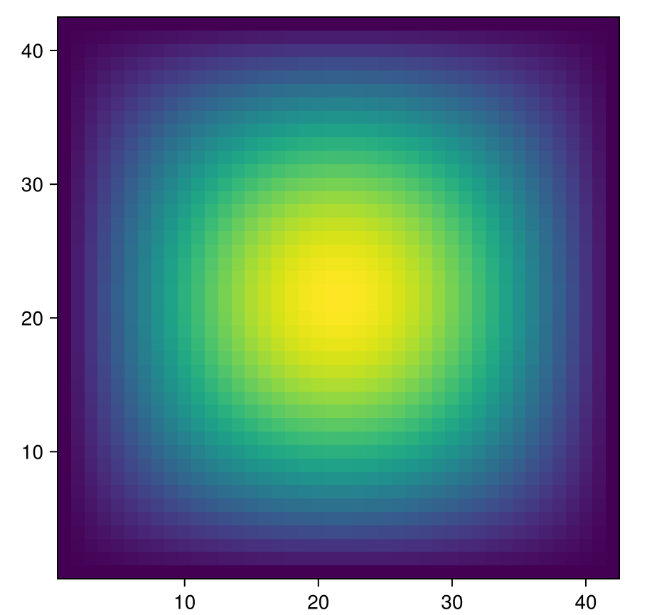
• Define our BC and source term functions: f = (x, y) -> sin(pi*x) * sin(pi*y); g = (x,y) -> 0.0
• Define the number of grid points in each direction in the interior: n_grid = 40
• Solve the Poisson equation: u = solve_poisson(f, g, n)
• Convert the solution to a matrix: u_mat = reshape_solution(u, n_grid)
• u_mat does not include the values at the boundaries, so we construct the full field: u_full = zeros(n_grid+2,n_grid+2)
• We fill it with u_mat values in the interior: u_full[2:end-1,2:end-1] = u_mat
• We then fill the boundary values of u_mat:
  • h = 1.0 / (n_grid + 1); u_full[1,:] = [g((i-1)*h, 0.0) for i in 1:n_grid+2]
  • u_full[end,:] = [g((i-1)*h, 1.0) for i in 1:n_grid+2]
  • u_full[:,1] = [g(0.0, (i-1)*h) for i in 1:n_grid+2]
  • u_full[:,end] = [g(1.0, (i-1)*h) for i in 1:n_grid+2]
• Plot the solution: fig = Figure(); ax = Axis(fig[1,1], aspect = 1); heatmap!(ax, u_full); fig

2.5 Adding documentation

Next, let’s add documentation to the functions in the project; see also the Documenter.jl guide. First, create a docs directory. Assuming you are using Julia v.1.12+, add the following to the Project.toml file:

[workspace]
projects = ["docs"]

Next, start a Julia REPL in the docs by calling julia --project=docs, enter pkg> mode with the ] key and install Documenter and JuFD26 by typing add Documenter and dev . (adding development version of base package). Add a src subdirectory to docs and create a make.jl file. in docs with the following code:

using Documenter, JuFD26

makedocs(sitename="JuFD26", remotes = nothing)

Trying to run this (by navigating to docs, and running julia --project=. make.jl) will fail, since no files are present in src/, but we can now add documentation to the functions in the project.

Add the following docstrings before the functions in src/solver.jl:

"""
    construct_matrix(n::Int)

Construct the finite difference matrix for the 2D Poisson equation on [0,1]x[0,1]
with Dirichlet boundary conditions.

Parameters:
- n: number of interior points in each direction (total grid is (n+2)x(n+2))
- h: grid spacing (1/(n+1))

Returns:
- A: sparse matrix representing the discrete Laplacian
"""


"""
    construct_rhs(f, g, n::Int)

Construct the right-hand side vector for the Poisson equation.

Parameters:
- f: function f(x,y) giving the RHS
- g: function g(x,y) giving Dirichlet boundary conditions
- n: number of interior points in each direction
- h: grid spacing (1/(n+1))

Returns:
- b: vector of length n*n containing the RHS values
"""

"""
    solve_poisson(f, g, n::Int)

Solve the 2D Poisson equation -Δu = f with Dirichlet boundary conditions u=g.

Parameters:
- f: function f(x,y) giving the RHS
- g: function g(x,y) giving Dirichlet boundary conditions
- n: number of interior points in each direction

Returns:
- u: solution vector of length n*n
"""

"""
    reshape_solution(u::Vector, n::Int)

Reshape the solution vector into a 2D grid for visualization.

Parameters:
- u: solution vector of length n*n
- n: number of interior points in each direction

Returns:
- U: n x n matrix representing the solution
"""

Next, create a file docs/src/index.md and add the following to the file:

# JuFD26

This is a finite difference code for solving the Poisson equation on a unit square.

## Public API

```@docs
solve_poisson
reshape_solution
```

## Private API

```@docs
JuFD26.construct_matrix
JuFD26.construct_rhs
```

Modify the docs/make.jl file to include the following:

makedocs(sitename="JuFD26", remotes = nothing,
         pages = [
        "Home" => "index.md",
        ])

You can have multiple pages, but for now, one is sufficient. Run julia --project=. make.jl from docs, and a build directory should be produced. To view the documentation, open docs/build/index.html in your browser (or alternatively, navigate to docs/build, run python3 -m http.server, and open the link).

2.6 Setting up Gitlab CI

First, make sure that Manifest.toml and docs/build have been added to .gitignore.

Next, you need to create a .gitlab-ci.yml file in the root directory of your project. This file will contain the instructions for Gitlab CI to build your documentation. You also need an NRW Gitlab account - create an empty remote repository there, and push the JuFD26 code to it.

Add the following to .gitlab-ci.yml:

stages:          # List of stages for jobs, and their order of execution
  - test

default:
  image: julia:1.12

unit-test-job:   # This job runs in the test stage.
  stage: test    # It only starts when the job in the build stage completes successfully.
  script:
    - echo "Running unit tests..."
    # Let's run the tests. Substitute `coverage = false` below, if you do not
    # want coverage results.
    - julia -e 'using Pkg; Pkg.activate("."); Pkg.instantiate; Pkg.test(coverage = true)'
    # Comment out below if you do not want coverage results.
    - julia -e 'using Pkg; Pkg.activate("."); Pkg.add("Coverage");
      using JuFD26; cd(joinpath(dirname(pathof(JuFD26)), ".."));
      using Coverage; cl, tl = get_summary(process_folder());
      println("(", cl/tl*100, "%) covered")'

You can test the pipeline by pushing to the NRW Gitlab.

Now we add another stage to stages which we will name deploy:

stages:          # List of stages for jobs, and their order of execution
  - test
  - deploy

We will add a job to the deploy stage which will build and deploy the documentation:

build-docs-job:
  stage: deploy
  script:
      - julia -e 'using Pkg; Pkg.activate("."); Pkg.instantiate; Pkg.add("Documenter")';
      - julia --color=yes --project=. docs/make.jl # make documentation
      - mv docs/build public # move to the directory picked up by Gitlab pages
  artifacts:
    paths:
      - public
  only:
      - main
  pages: true

Once the pipeline has been successfully executed, under Deploy/Pages in Gitlab one should see an active deployment.

An example of the project can be found at: https://gitlab.git.nrw/georgii.oblapenko/jufd26/ The gitlab pages documentation can be found at: https://jufd26-57cab6.pages.git.nrw

3 Python

A similar approach can be taken in Python, see https://gitlab.git.nrw/rwth-acom/teaching/pyfd26 for an example repository.

3.1 Structure

The structure of the repository is as follows:

.
├── docs
│   ├── api.md
│   └── index.md
├── examples
│   ├── plot_two_source_terms.py
│   └── README.md
├── mkdocs.yml
├── pyproject.toml
├── README.md
├── src
│   ├── pyfd26
│   │   ├── __init__.py
│   │   └── solver.py
└── tests
    └── test_solver.py

3.2 Installation

python -m venv .venv
source .venv/bin/activate
python -m pip install --upgrade pip
python -m pip install -e .[docs]
python -m unittest discover -s tests -v

creates a virtual environment, activates it, installs the package in editable mode with the documentation dependencies, and runs the tests.

An alternative approach is to use conda (or work globally).

3.3 Important Files

The src/pyfd26 directory contains the code.

__init__.py:

"""Public package interface for the finite-difference Poisson solver."""

from .solver import construct_matrix, construct_rhs, reshape_solution, solve_poisson

__all__ = [
    "construct_matrix",
    "construct_rhs",
    "reshape_solution",
    "solve_poisson",
]

solver.py:

# ...
def construct_matrix(n: int):
    # ...

pyproject.toml:

[build-system]
requires = ["setuptools>=69", "wheel"]
build-backend = "setuptools.build_meta"

[project]
name = "pyfd26"
version = "0.1.0"
description = "Finite-difference Poisson solver on the unit square."
readme = "README.md"
requires-python = ">=3.11"
authors = [
  { name = "Lambert Theisen", email = "lambert.theisen@rwth-aachen.de" },
]
license = "MIT"
keywords = ["finite differences", "poisson equation", "teaching", "pde"]
dependencies = [
  "numpy>=1.26",
]
classifiers = [
  "Development Status :: 3 - Alpha",
  "Intended Audience :: Education",
  "Programming Language :: Python :: 3",
  "Programming Language :: Python :: 3.11",
  "Programming Language :: Python :: 3.12",
  "Programming Language :: Python :: 3.13",
  "Topic :: Scientific/Engineering :: Mathematics",
]

[project.optional-dependencies]
docs = [
  "mkdocs>=1.6",
  "mkdocstrings[python]>=0.29",
]
examples = [
  "matplotlib>=3.8",
]

[tool.setuptools]
package-dir = {"" = "src"}

[tool.setuptools.packages.find]
where = ["src"]

mkdocs.yml:

site_name: pyfd26
site_description: Finite-difference Poisson solver documentation
repo_url: https://gitlab.git.nrw/rwth-acom/teaching/pyfd26

theme:
  name: readthedocs

nav:
  - Home: index.md
  - API: api.md

plugins:
  - search
  - mkdocstrings:
      handlers:
        python:
          options:
            docstring_style: google
            show_root_heading: true
            show_source: false

markdown_extensions:
  - admonition
  - toc:
      permalink: true

.gitlab-ci.yml:

stages:
  - test
  - deploy

default:
  image: python:3.13

variables:
  PIP_CACHE_DIR: "$CI_PROJECT_DIR/.cache/pip"

cache:
  paths:
    - .cache/pip

test:
  stage: test
  before_script:
    - python -m pip install --upgrade pip
    - python -m pip install -e . coverage
  script:
    - coverage run -m unittest discover -s tests -v
    - coverage report -m
    - coverage xml
  artifacts:
    when: always
    paths:
      - coverage.xml
  coverage: '/TOTAL\s+\d+\s+\d+\s+(\d+%)/'

pages:
  stage: deploy
  before_script:
    - python -m pip install --upgrade pip
    - python -m pip install -e .[docs]
  script:
    - mkdocs build --strict --site-dir public
  artifacts:
    paths:
      - public
  rules:
    - if: '$CI_COMMIT_BRANCH == $CI_DEFAULT_BRANCH'

3.4 References

• python.org Packaging

4 Questions

• What is the expected convergence rate of the finite difference method for the Poisson equation? How can we verify it?
• How can we modify the code to solve the Poisson equation on a rectangular domain instead of a unit square?
• How can we modify the code to solve the Poisson equation on a non-uniform grid?
• How can we modify the code to solve the Poisson equation in 3D?